Numerical Simulations of Fractional Gaussian Fields
I describe the basic properties of fractional Gaussian fields and show some numerical simulations.
Fractional Gaussian fields (FGFs) are a canonical example of random fields. They are spatial versions of the fractional Brownian motion, a stochastic process with self-similar and correlated increments, which is characterized by a parameter $H$, called the Hurst exponent. The Hurst exponent is a measure of autocorrelations in a series. If it is between 1/2 and 1, there is positive autocorrelation in the series, meaning that high values are usually followed by high values, while if it is between 0 and 1/2, there is negative autocorrelation, and the values oscillate strongly. If $H=1/2$, successive values are independent, and the fractional Gaussian field coincides with Brownian motion. Let us define a scalar random field $u(x)$ for in $x \in \mathbb{R}^d$ by
\[u_H(x) = \int_{\mathbb{R}^d} e^{2\pi i k \cdot x} \frac{1}{\lvert k \lvert^{H+d/2}_{1/L}} \widehat{dW}(k) \ ,\]where $\lvert k \lvert_{1/L}$ denotes a regularized norm over small wavelengths $k$, meaning that $\lvert k \lvert_{1/L} \approx 1/L$ for small $k$ and $\lvert k \lvert_{1/L} \approx \lvert k \lvert$ for large $k$. One possible choice for this regularization is $\lvert k \lvert_{1/L} = \sqrt{k \cdot k + 1/L^2}$. The increment of a white noise field is denoted by $dW$ and its Fourier transform by $\widehat{dW}$.
The statistics of this random field is Gaussian, as is clear from its name and definition, since we have an integral over Gaussian random variables (white noise). To characterize it, we can look at the power spectrum,
\[E(k) = \int d\Omega \, k^{d-1} \mathbb{E}\lvert \hat u_H \lvert^2 \ ,\]where $d\Omega$ is the surface area element in $d$-dimensions, and the second order structure function ($\mathbb{E} \lvert \delta_{\ell} u_H \lvert^2$), where the increment is defined as
\[\delta_{\ell} u_H(x) = u_H(x+\ell e_i) - u_H(x)\]for some unit vector $e_i$.
The power spectrum, for large wavelengths, decays as
\[E(k) \sim c_H \, k^{-2H-1}\]and for the structure function we observe an inertial range where
\[\mathbb{E} \lvert \delta_{\ell} u_H \lvert^2 \sim d_H (\ell/L)^{2H} \ .\]At large separation, there is no correlation and we observe the asymptotic value of twice the variance.
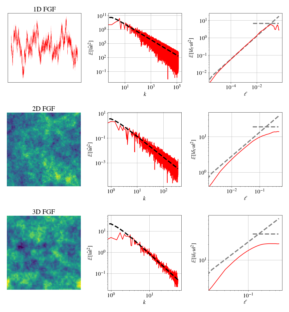
In the figure below are the results of the numerical simulations together with visualizations of the random series in one, two and three dimensions. In the center column the power spectrum is shown, together with its analytical result (black dashed line), and in the right column, the second order structure function, together with analytical results for the inertial range (dashed slope) and the variance (dashed horizontal line). In all cases, I chose $H=1/3$, a value that is important in the context of turbulence. For the grid sizes, $N=2^{18}$ points were used in 1D, $N=2^9$ in each direction in 2D and $N=2^6$ in each direction in 3D. At higher dimensions the numerical simulations require much more memory and processing power, and this can be seen especially in the structure functions, which are close to the analytical values, but still differ. For larger $N$, these differences would be smaller. In 3D, only a two-dimensional cross section is shown, and we can see that its resolution is smaller as well.

These random fields were generated in the C language with the FFTW library and the data was analyzed in Python. The code is available on Github.
For a further reading on Gaussian random fields and their properties the reader may consult
- Frisch, U. (1995). Turbulence. Cambridge university press. A classic textbook on the phenomenology of turbulence.
- Random fields. Lecture notes by Jonathan Taylor.
- Reneuve, J., & Chevillard, L. (2020). Flow of spatiotemporal turbulentlike random fields. Physical Review Letters, 125(1), 014502.. This paper and its supplementary material detail some applications of random fields to hydrodynamic turbulence.