Time scales in the pseudospectral simulation of the heat equation
This is a discussion of a pseudospectral simulation of the stochastically forced heat equation and an analysis of the time scales needed for the results to converge.
The heat equation is a classic model which describes, for instance, diffusion of heat in a surface with a certain initial temperature profile. It is a linear equation, with an analytical solution, which will greatly aid us in understanding the pseudospectral simulation. Consider the one-dimensional scalar field $u$, which depends on space $x$ and evolves in time $t$. It is governed by \begin{equation} \frac{\partial u}{\partial t} = \alpha \frac{\partial^2 u}{\partial x^2} + f \ , \end{equation} where $\alpha$ is the diffusivity constant and $f$ is an external stochastic force, of Gaussian statistics, which we define by its zero mean
\[\mathbb{E}[f(t,x)] = 0\]and its two-point correlation function,
\[\mathbb{E}[f(t,x) f(t',y)] = \delta(t-t') C_f(x-y) \ .\]Since the correlation function $C_f$ depends only on the difference $x-y$, $f$ is statistically homogeneous.
One way to do a numerical simulation of this PDE is with the method of finite differences, where we partition space into slices with separation $\delta x$ and time with intervals $\delta t$. One can show with von Neumann stability analysis that the explicit algorithm for finite differences is only stable for
\[r = \alpha \frac{\delta t}{\delta x^2} < 1/2 \ .\]This constant is obtained with a centralized prescription for the spatial derivatives, but other explicit schemes would give equivalent results, and only the constant would change.
Let us now look at an explicit scheme with a pseudospectral method. In this approach, we simulate the evolution of the Fourier modes of $u$. For the computation of nonlinearities, which are often localized in real space, Fast Fourier Transforms (FFTs) are used to port the $u$ field to real space and back to Fourier space in an efficient manner. The heat equation is linear, hence we will only need FFTs in order to measure some observables in real space.
In Fourier space, the heat equation (1) is
\[\frac{\partial \widehat u}{\partial t} = - 4 \pi^2 \alpha k^2 \widehat u + \widehat f\]where the adopted convention for the Fourier transform is
\[\mathcal{F}[u](t, k) \equiv \widehat{u}(t, k)=\int_{\mathbb{R}} e^{-2 i \pi k x} u(t, x) d x \ .\]It can be noticed this equation is equivalent to an Ornstein-Uhlenbeck process for each Fourier mode $\widehat u(\cdot,k)$, except for $k=0$. In the Ornstein-Uhlenbeck equation,
\[\frac{d v}{d t} = - \frac{v}{T} + \sigma f \ ,\]the drift constant $1/T$ defines a typical time for the system. For white-in-time forcing, the solution reaches a statistically stationary state within a time of the order of $T$. This is what happens independently to each Fourier mode of the heat equation. Furthermore, since $f$ is homogeneous, the Fourier modes of the forcing are also independent. This can be seen in the following correlation function:
\[\mathbb{E}[\widehat{f}(t,k)\widehat{f^*}(t',k')] = \delta(t-t') \delta(k-k') \widehat{C}_f(k) \ .\]To numerically solve the heat equation with a pseudospectral method, all of these Ornstein-Uhlenbeck processes for different Fourier modes must be well resolved. This means that the time step $\delta t$ must be smaller than the smallest drift time scale and the total time of the simulation must be big enough so that the largest drift time scale is also captured.
Some other details are needed for the numerical simulation: The solution is periodic, and is discretized in a box of total size $L_{\mathrm{total}}=1$, with $N$ grid points in space, regularly spaced. Each Fourier mode then has a corresponding wavenumber of
\[k_i = i/L_{\mathrm{total}} \ , \text{for $0 \leq i \leq N/2$, and}\] \[k_i = -(N-i)/L_{\mathrm{total}} \ , \text{for $N/2 \lt i \lt N$.}\]Considering the Fourier modes with $k\neq 0$, the smallest time scale is the one with largest wavenumber ($i=N/2$),
\[T_{k=N/2} = \frac{1}{\pi^2 \alpha N^2} \ ,\]and the largest time scale is the one with smallest wavenumber,
\[T_{k=1} = \frac{1}{4 \pi^2 \alpha} \ .\]Based on this time scale analysis, we see that the time steps of the algorithm must be smaller than $T_{k=N/2}$. Since $\delta x = L_{\mathrm{total}}/N$, we find that
\[\delta t < \frac{(\delta x)^2}{\pi^2 \alpha L_{\mathrm{total}} } .\]This conclusion is very similar to the one reached by the stability requirement of the explicit finite difference algorithm: We see the same dependence in $(\delta x)^2/\alpha$. A stability analysis of the equation $dv/dt = -\alpha v$ (the deterministic part of the Ornstein-Uhlenbeck equation) gives an equivalent result and can be found in these lecture notes. Also notice that the actual value of $\delta t$ must be significantly smaller than the bound obtained from a stability analysis. In the simulations I’m going to show next, I used $\delta t = 0.12 (\delta x)^2 / (\pi^2 \alpha L_{\mathrm{total}})$. This happens because we not only need the algorithm to be stable, but we also need it to be accurate: it must reproduce well the real solution of the equation.
Now I’m going to show the results of a numerical simulation. It was done with $N=2^9$ grid points and the statistical results are averages over 200 independent realizations. The code was written in C with the FFTW library for the Fast Fourier Transforms and is available on Github.
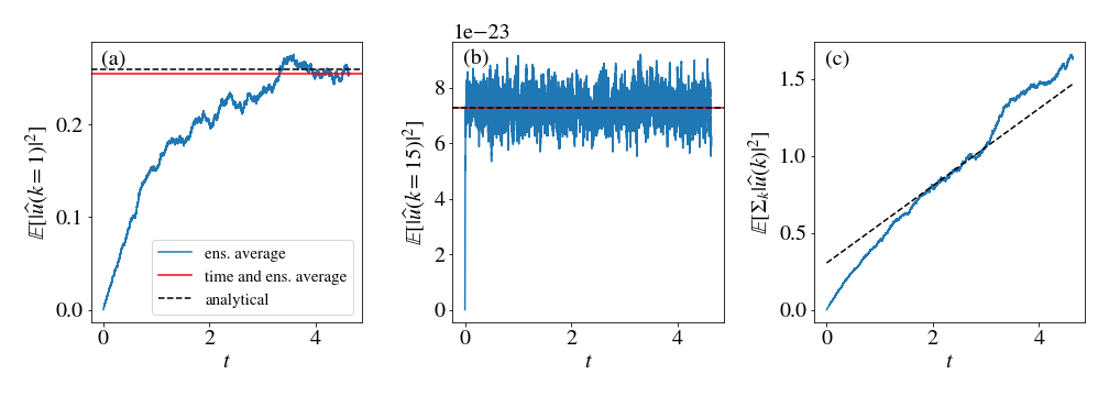
To compare the simulation with the analytical solutions, I measured the variance of individual Fourier modes, as can be see in the figure above. On the left (a), the variance of $\widehat{u}(k=1)$ is shown. It is a low wavenumber mode, and it has a big typical time $T_{k=1}$, hence it takes a long time to reach a stationary state. On the center (b), the wavenumber $k=15$ is shown and its the stationary state is reached much faster. In blue, I’m showing the average of 200 realizations, in black dashed lines the analytical result (in the stationary state). For the red line, I took an average in time and on the ensemble, considering only the stationary state, and it can be seen that the analytical result and the average in time are in close agreement. In (c), I’m showing the total variance of the Fourier modes, $\sum_k \mathbb{E}[|\widehat{u}(t,k)|^2]$, including $k=0$, which does not reach a stationary state, but grows linearly with time. The ensemble average, in blue, is compared to the analytical result, in a black dashed line, and it can be seen that both agree well. After a long time, the simulation starts to lose accuracy and the curves start to diverge.
Notice that the results in the first figure only involved Fourier modes and their sums, hence they can be compared to the analytical results for any number of grid points, big or small. Let us now look at some results in real space and compare them to analytical results in the continuum. Now a big number of grid points will be needed, so that results in the continuum are reproduced by the discrete numerical simulations.
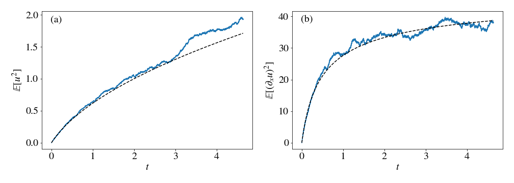
On the left (a), I measured the variance of the $u$ field in real space and compared it with the analytical result, which grows as a square root of $t$. On the right (b), I’m showing the gradient of $u$ and its analytical result. Both results match very well their continuum analogues. The variance also diverges at some large time, where the simulation is no longer accurate. To resolve even longer times, we would need a smaller timestep and a larger grid.
The analytical results can be obtained directly from the solution of the heat equation, which is
\[u(t,x) = \int_{\mathbb{R}} dk \int_0^t ds \, e^{2\pi i k x} e^{-4 \pi^2 \nu k^2 (t-s)} \widehat{f}(s,k)\]Using \(C_f(x) = e^{-x^2/2 L^2}\) for the forcing correlation function, we find that the variance of $u$ is
\[\mathbb{E}[u^2] = \frac{L^2}{2 \nu} \left( \sqrt{1+\frac{4 \nu t}{L^2}} - 1 \right)\]and the variance of its gradient reaches a stationary limit at infinite time
\[\lim_{t \to \infty} \mathbb{E}[(\partial_x u)^2] = \frac{1}{2 \nu} \ .\]This simple equation with an analytical solution can be used as a test for the code, and as a way to understand the timescales involved in the pseudospectral algorithm. It serves as the first step to nonlinear problems, which are more complex and very often don’t have analytical solutions.
For a further reading on the stochastic heat equation, the reader may consult
- Walsh, J. B. (1986). An introduction to stochastic partial differential equations. This classic paper discusses the mathematical properties of linear PDEs with an external noise, such as the heat equation.
- Chevillard, L. Une peinture aléatoire de la turbulence des fluides (2015) (in french) This text revisits the stochastic heat equation problem under the light of the phenomenology of turbulence and rough random fields.
- Slides by Yimin Xiao. Lecture slides on random fields